Anomaly-Detection with Transformers Machine Learning Architecture
Anomaly Detection
Anomaly Detection refers to the problem of finding anomalies in (usually) large datasets. Often, we are dealing with time-dependent or at least sequential data, originating, for example, from logs of a software or sensor values of a machine or a physical process. Anomalies are parts of such a time-series which are considered as not normal. For example, because they have been collected from a machine suffering a degradation. By detecting anomalies automatically, we can identify problems in a system and can take actions before a larger damage is inflicted.
There are various established techniques to detect anomalies in time-series data, for example, dimension reduction with principal component analysis. Recently, deep-learning techniques are applied to the detection of anomalies as well. For an overview, see this survey. Typically, some form of sequential model (e.g. Long-Short-Term-Memory or Gated-Recurrent-Unit) are applied for this task. These types of models are similar to models that have been used in text-analysis and natural language processing (NLP). This is not much of a surprise as text is also a form of sequential data with many complex interdependencies. In the last years, major improvements have been made on using deep-learning techniques for NLP, which resulted in models that are, for example, translate text in a way nearly indistinguishable from human translations. A type of architecture which is the base for many current state-of-the-art language models is the transformer architecture. The transformer architecture leverages several concepts (such as encoder/decoder, positional encoding and attention), which enables the respective models to efficiently cope with complex relationships of variables especially with long-ranging temporal dependencies (e.g. due to delay in physical processes). In this paper we demonstrate how the transformer architecture can be deployed for anomaly detection.
Transformer Deep-Learning Architecture
For the anomaly detection we employ the popular transformer architecture that has been successful especially in the field of natural language processing and excels especially in transforming sequences. The transformer architecture uses an encoder to compress an input sequence into a fixed size vector capturing the characteristics of the sequence. Then it uses a decoder to construct the output sequence from the compressed representation. What makes the transformer architecture different from other encoder-decoder architectures is the fact that it uses no variant of recurrent network (such as long-short-term-memory) and instead captures dependencies between different time instants by a preprocessing technique called positional encoding together with an architecture pattern called attention.
For the task of anomaly detection, we use the transformer architecture in an autoencoder configuration. The idea is to train the model to compress a sequence and reconstruct the same sequence from the compressed representation. As the model will be trained on system runs without error, the model will learn the nominal relationships within a system run (e.g. relationships between sensor values). Hence, we can use the difference between the input sequence and the reconstruction sequence – the so called reconstruction error – as a measure for anomaly.
Figure 1: High-Level Overview over the transformer architecture
Running Example
For this paper, we use as a running example a controlled cooling process. The process models the situation where an object needs to be kept at a constant temperature (e.g. a processor in a computer). However, there is a dynamically changing heat-flow from a different physical process (e.g. due to inner workings of the processor). In order to keep the object at a constant temperature a cooling facility is installed. This facility pumps cool water of a constant temperature around the object. By controlling the amount of water that is pumped around the object, the system can apply a stronger or weaker cooling effect. In order to efficiently control this process, a temperature sensor is installed and connected with a PID controller which controls the water pipe. However, the system can suffer from two problems. First, the pipe that transports water from the pump to the object can get clogged over time, leading to reduced flow of water. Second the temperature sensor can deteriorate leading to delayed sensor readings. We modelled this system in the physics modelling environment OpenModelica to generate evaluation data for our approach.

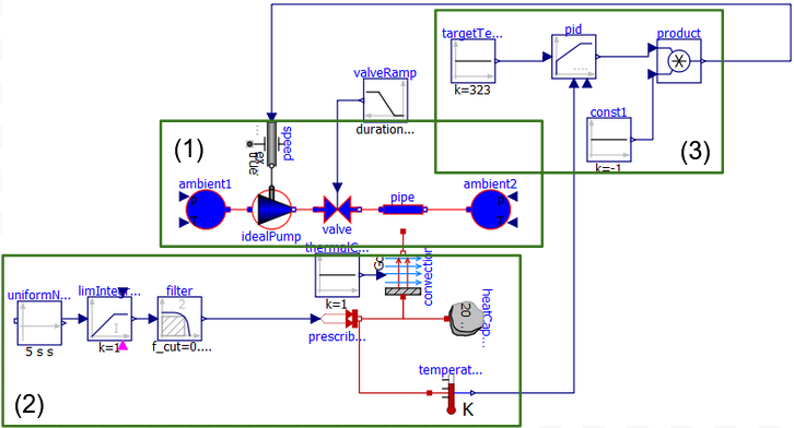
Figure 2: OpenModelica model for the cooling system
The OpenModelica model is based on the „Pump and Valve“ example model from OpenModelica.
In the centre (1) is the pumping pipeline that models pumping water from one reservoir to another via a pump. The speed of the pump can be externally controlled. In order to model a gradually clogging system, we inserted a valve between the pump and the pipe.
The lower part (2) models the heating pipeline. The centre of this part is the object to be kept cool, modelled as a heat capacitor. The heat capacitor is heated up by a heat-flow and cooled down via convection from/to the water pipe. The heat flow is generated in random fashion modelling e.g. a random workload of the computing processes (if we take the object as a cpu processor).
The upper right part (3) is the controller that receives readings of a temperature sensor and controls the speed of the pump to maintain the optimal temperature.
Additionally, there is a ramp block attached to the valve in order to model the gradual clogging of the pipe via the valve. In our experiments, we simulate clogging the pipe up to 25% over 14 hours.
Figure 2 shows a sample run of the nominal system without errors as simulated in OpenModelica. We only depict three process variables:
- prescribedHeafFlow.Q_flow: The external heat source, which his generated randomly
- idealPump.V_flow: The water flow measured at the pump
- heatCapacitor.T: The temperature of the object in °C
As you can see, the temperature is mostly at the desired temperature of 50°C. However, sometimes the heat flow cumulates such that the system cannot maintain the temperature any more, even with maximal cooling. In these cases, the temperature rises a few degrees above 50°C. Figure 3 shows the same part of the simulation run, however this time with a gradually clogging pipe. Due to the clogged pipe the cooling capacity of the system is reduced which results in more frequent phases of overly high temperature. The temperature in these phases also raises slightly higher. Additionally, observe that the water flow through the pipe is gradually lowering. If you compare the two runs, you see that the two runs are mostly similar and the differences are very subtle.
In order to train the transformer model, we generated three datasets
- CS-Train: Simulation data equivalent to 14 days without any clogging. One data-point roughly every 5 seconds, which means 1,019,035 datapoints in total.
- CS-Val-Nom: Simulation data equivalent to 1 day without any clogging. One data-point every 5 seconds. Note that this dataset is generated from a different random heating profile compared to CS-Train.
- CS-Val-Clogged: Simulation data equivalent to 1 day with clogging rising from 0% to 25% during the first 14 hours. One data-point every 5 seconds. Note that this dataset is generated from the same heating profile as CS-Val-Norm.
Figure 3: Simulation run of the model (without anomalies)
Figure 4: Simulation run of the model with a clogged pipe
Evaluation
For the training we standardized the CS-Train dataset by subtracting the mean and dividing by the standard deviation for each feature separately in order to have comparable scales for all features. Then we subdivided the data into runs of 90 datapoints each (i.e. equivalent to roughly 7.5 minutes). We split the data into runs such that two adjacent runs overlap by 80 datapoints. Finally, we grouped the runs into mini-batches of length 64. We trained the transformer using this dataset for 20 epochs using the mean absolute error between input data and reconstruction data as loss function.
In order to validate the performance of the trained model we use the two other datasets, which we standardized and split into runs of 90 datapoints in the same way as the training dataset. For each dataset we calculated the mean absolute error between the input and the reconstructed output as measure for the degree of anomaly.
For CS-Val-Nominal (containing a simulation run of the system without clogging, but with a different random heating profile compared to the training set) we expect an overall low value of the reconstruction error. For CS-Val-Clogged we expect the reconstruction error to be low at the early runs and then rise gradually over time.
When looking at the results depicted in Figure 5 we see the expected pattern. The charts show the reconstruction error as measure for anomaly and the average reconstruction error over the four last datapoints. Additionally, from an additional nominal system run we derived a threshold for anomalies. This threshold is choses such that 97.5% of the reconstruction errors in a nominal system run lie below the threshold. As is visible in the figure, in the nominal system run the reconstruction error is below the threshold for all except one instance. The average reconstruction error is below the threshold for the whole time-span. In case of the clogged system run, the reconstruction error is gradually rising and after around half the time-span the average is consistently above the threshold. This matches closely the (simulated) physical reality.
Figure 5: Reconstruction errors for the nominal and the clogged run
Summary
In this paper, we showed that the transformer Deep Learning architecture, which proved to be effective for Natural Language Processing tasks, is able to detect subtle anomalies in physical systems. As an example we used data generated from a simulated cooling system with a random heating profile. Already with few learning cycles the system was able to recognize the gradual clogging of a pipe, although it has never seen such a behavior before.
If that sounds interesting to you, are you want to get started with anomaly detection or other applications for machine learning or text analytics, feel free to contact me (maximilian.junker@qualicen.de)
Sorry, the comment form is closed at this time.


Shreejal
04/02/2021Hey,
Can you share the transformer Autoencoder model definition for sequence reconstruction?
Maximilain
15/02/2021Hi Shreejaal, yes I can share the code, I have to dig it out though and probably add a few comments 🙂 give me a couple of days…
Said
26/02/2021I’m also intrested in the code and model definition, thank you!
niv d
02/05/2021I would love to get the code and model definition too.
Thank you!
sam
15/06/2021Hi.. can you share the code?
Lahm
08/07/2021I’m interested as well